10 Medians and Resampling (Ch. 10)

Create a dataset to approximate the data underlying Drennan’s Table 10.1.

ClassicSites<-read.csv("data/Drennan_datasets/AllClassic.csv", 
                   header=T)[,-1] #[,-1] removes extraneous leading column of rownames

Compare Early Classic and Late Classic site areas with a boxplot, and by measures of central tendency. For the latter we can use the handy aggregate() function, which like boxplot() can take a formula input (the first use of aggregate() below can be read as “aggregate area by period, then calculate the mean for each group”).

boxplot(Area ~ Period, data = ClassicSites, names = c("Early Classic", "Late Classic"),
        ylab = "Area (ha)", boxwex = .25, col = "orange", outpch = 21, outbg = "orange")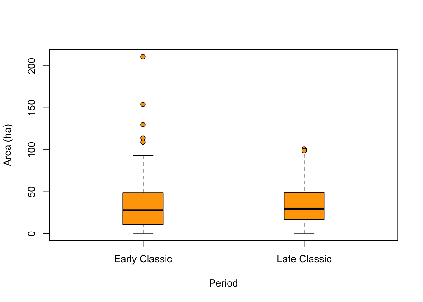

aggregate(Area ~ Period, data = ClassicSites, mean)

##          Period     Area
## 1 Early Classic 35.79646
## 2  Late Classic 35.18421

aggregate(Area ~ Period, data = ClassicSites, median)

##          Period Area
## 1 Early Classic   28
## 2  Late Classic   30

Bootstrap the median area of Early Classic sites, 10000 repetitions (using our old friend sapply()). Note how easy (and fast) it is to do this 10000 times, and think about what doing that by hand would look like; this is why resampling has become a more viable technique in the last few decades.

EClassic <- ClassicSites[ClassicSites$Period == "Early Classic",]
MedianBootstrap <- sapply(1:10000, function(x) median(sample(EClassic$Area, replace = T)))  

#then plot a histogram of the results
hist(MedianBootstrap, breaks = 18, col = "grey", main = "", xlab = "Area medians (ha)")
#add vertical lines showing the medians of both bootstrapped samples and actual sites
abline(v = median(MedianBootstrap), col = "blue", lwd = 2)
abline(v = median(EClassic$Area), col = "red", lty = 2, lwd = 2)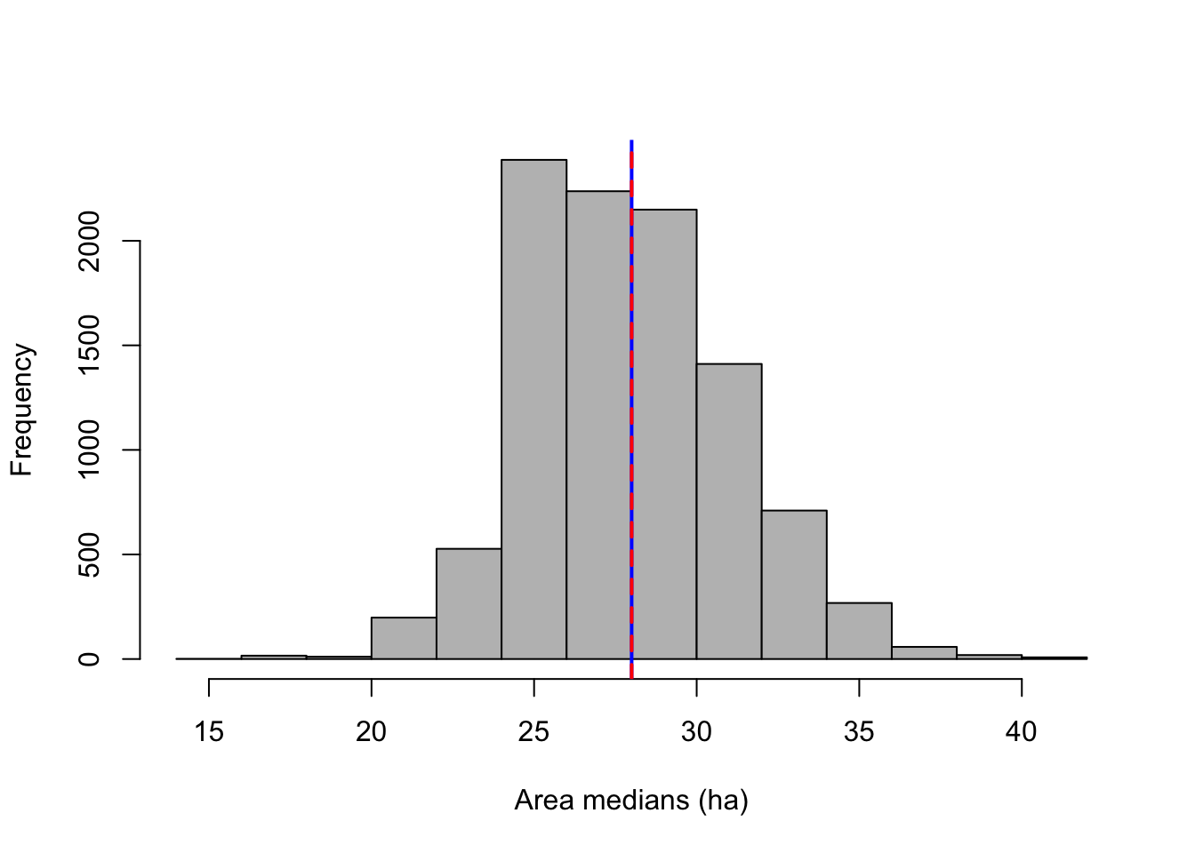

We can calculate percentiles (to use as confidence intervals) using quantile().

quantile(MedianBootstrap, p=c(.01, .025, .05, .95, .975, .99))     

##    1%  2.5%    5%   95% 97.5%   99% 
##    22    23    24    34    35    36

Using the .05 and .95 percentiles, then, we can be 90% confident that the population median lies between 24ha and 34ha.

Although we normally would use the Central Limit Theorem to find confidence intervals around the population mean, in principle we could bootstrap the mean too.

MeanBootstrap<-sapply(1:10000, function(x) mean(sample(EClassic$Area, replace = T))) 
hist(MeanBootstrap, breaks = 20) 
abline(v = mean(MeanBootstrap), col="blue", lwd = 2)
abline(v = mean(EClassic$Area), col = "red", lty = 2, lwd = 2)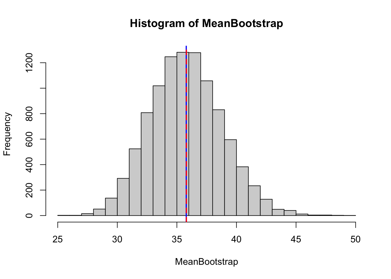

Resampling has become increasingly common as computers have made it practical; for more, see (here)[###addd link###]).