4 Comparing Batches (Ch. 4)
First make some useful data - post hole diameters at the Black and Smith sites.
BSPosts <- data.frame(Site = c(rep("Black Site", 13), rep("Smith Site", 15)),
                      Diameter = c(9.7, 9.2, 12.9, 11.4, 9.1, 44.6, 10.5, 11.7, 11.1,
                                 7.6, 11.8, 14.2, 10.8, 20.5, 17.2, 15.3, 15.9, 18.3,
                                 17.9, 18.6, 14.3, 19.4, 16.4, 18.8, 15.7, 18.9, 16.8,
                                 8.4))
head(BSPosts)
## Site Diameter
## 1 Black Site 9.7
## 2 Black Site 9.2
## 3 Black Site 12.9
## 4 Black Site 11.4
## 5 Black Site 9.1
## 6 Black Site 44.6## Site Diameter
## Length:28 Min. : 7.60
## Class :character 1st Qu.:11.03
## Mode :character Median :14.80
## Mean :15.25
## 3rd Qu.:18.00
## Max. :44.60#You already have some tools for comparing the two sites
by(BSPosts$Diameter, BSPosts$Site, summary)## BSPosts$Site: Black Site
## Min. 1st Qu. Median Mean 3rd Qu. Max.
## 7.60 9.70 11.10 13.43 11.80 44.60
## ------------------------------------------------------------
## BSPosts$Site: Smith Site
## Min. 1st Qu. Median Mean 3rd Qu. Max.
## 8.40 15.80 17.20 16.83 18.70 20.50#somewhat more thorough, using the 'Hmisc' package (if not particularly informative in this case)
by(BSPosts$Diameter, BSPosts$Site, Hmisc::describe) ## BSPosts$Site: Black Site
## dd[x, ]
## n missing distinct Info Mean pMedian Gmd .05
## 13 0 13 1 13.43 11.1 6.964 8.50
## .10 .25 .50 .75 .90 .95
## 9.12 9.70 11.10 11.80 13.94 26.36
##
## Value 7.6 9.1 9.2 9.7 10.5 10.8 11.1 11.4 11.7 11.8 12.9
## Frequency 1 1 1 1 1 1 1 1 1 1 1
## Proportion 0.077 0.077 0.077 0.077 0.077 0.077 0.077 0.077 0.077 0.077 0.077
##
## Value 14.2 44.6
## Frequency 1 1
## Proportion 0.077 0.077
##
## For the frequency table, variable is rounded to the nearest 0
## ------------------------------------------------------------
## BSPosts$Site: Smith Site
## dd[x, ]
## n missing distinct Info Mean pMedian Gmd .05
## 15 0 15 1 16.83 17.23 3.023 12.53
## .10 .25 .50 .75 .90 .95
## 14.70 15.80 17.20 18.70 19.20 19.73
##
## Value 8.4 14.3 15.3 15.7 15.9 16.4 16.8 17.2 17.9 18.3 18.6
## Frequency 1 1 1 1 1 1 1 1 1 1 1
## Proportion 0.067 0.067 0.067 0.067 0.067 0.067 0.067 0.067 0.067 0.067 0.067
##
## Value 18.8 18.9 19.4 20.5
## Frequency 1 1 1 1
## Proportion 0.067 0.067 0.067 0.067
##
## For the frequency table, variable is rounded to the nearest 0## BSPosts$Site: Black Site
## [1] 7.6 9.7 11.1 11.8 44.6
## ------------------------------------------------------------
## BSPosts$Site: Smith Site
## [1] 8.4 15.8 17.2 18.7 20.5Comparing things in more visual ways is often preferable, especially as datasets get larger. Drennan introduces box-and-dot plots as an important basic tool for this.
#Creating a box-and-dot plot (or boxplot) is easy, but aggregates all of our data.
boxplot(BSPosts$Diameter, notch = F, log = "", col = 8, ylab = "Diameter")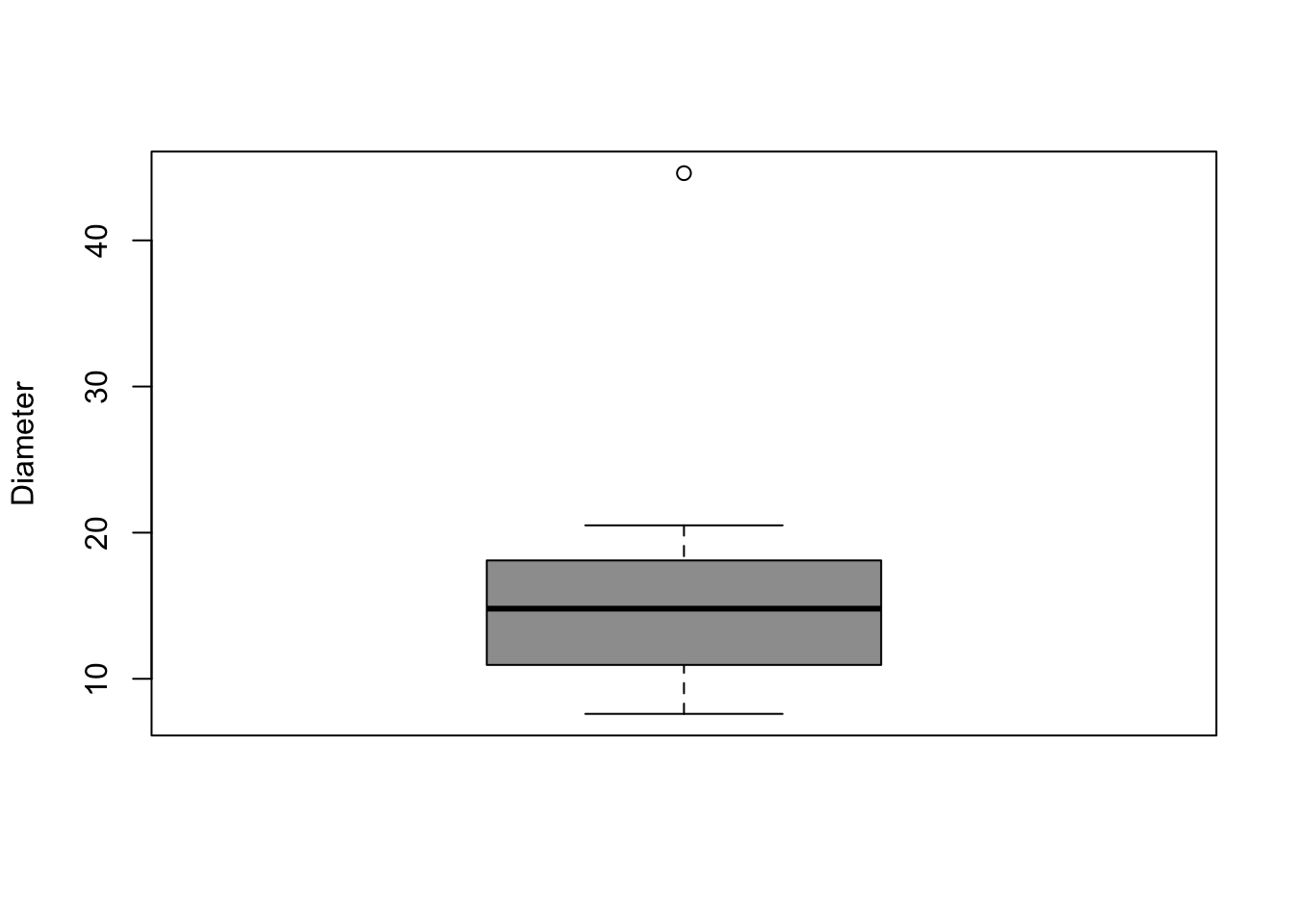
In Fig. 4.1 Drennan plots only post hole diameters from the Smith site, which we can replicate by doing some selection with [ on our BSPosts object. We can do this either by subsetting to create a new object and then using that in boxplot(), or by wrapping the subsetting step into our boxplot() command; both are illustrated here. The former is easier to read but involves more typing and contributes to the proliferation of objects in your working environment (note that if you don’t want these around, you can get rid of them using rm()).
SmithPosts <- BSPosts[BSPosts$Site == "Smith Site",]

boxplot(SmithPosts$Diameter, notch = F,
log = "", col = 8, ylab = "Diameter", ylim = c(6,28)) 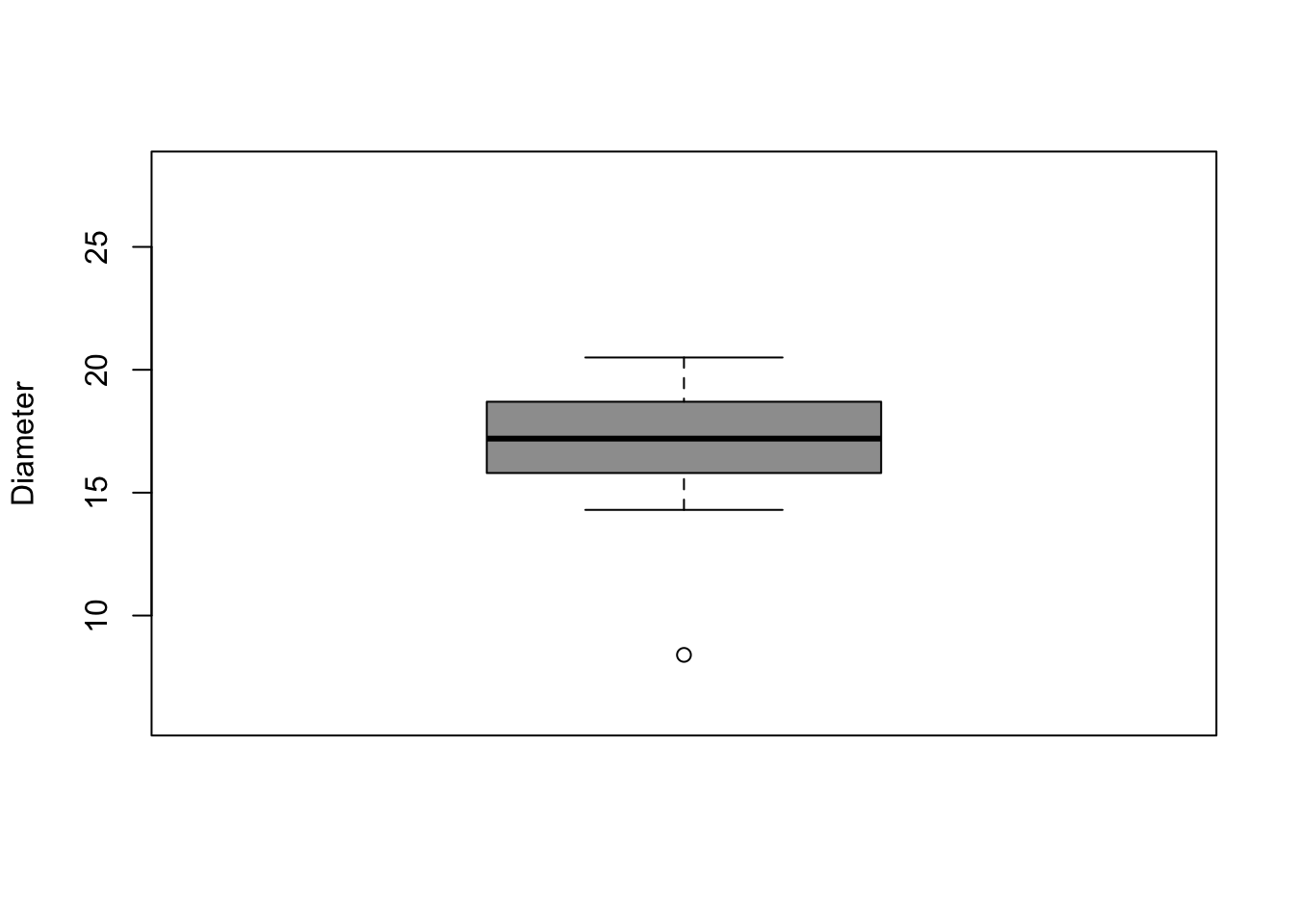
boxplot(BSPosts[BSPosts$Site == "Smith Site",]$Diameter, notch = F,
log = "", col = 8, ylab = "Diameter", ylim = c(6,28)) 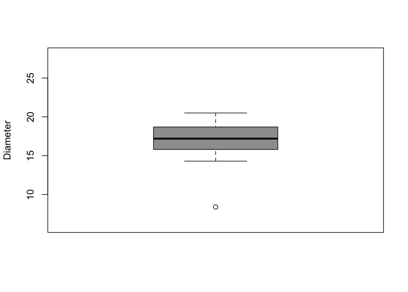
The y-axis will default to a bit more than the range of the data we’re plotting, so if (as Drennan does in Fig.4.1) we want to see the diameters from the Smith Site within the range of the whole dataset, we have to specify the ylim parameter (c(6,28) above creates a two-item vector in which the first element is used as the minimum and the second as the maximum).
Of course, the point is to compare different sites, as Drennan does in Fig. 4.2. Note the “formula” input (Diameter ~ Site), which refers to columns/variables of the data frame specified in the data argument. The formula should be read as “diameter by site” - that is, diameter on the y-axis and site on the x-axis.
#use the '~' operator
boxplot(Diameter ~ Site, data = BSPosts, col = 8, xlab = "Site", ylab = "Diameter")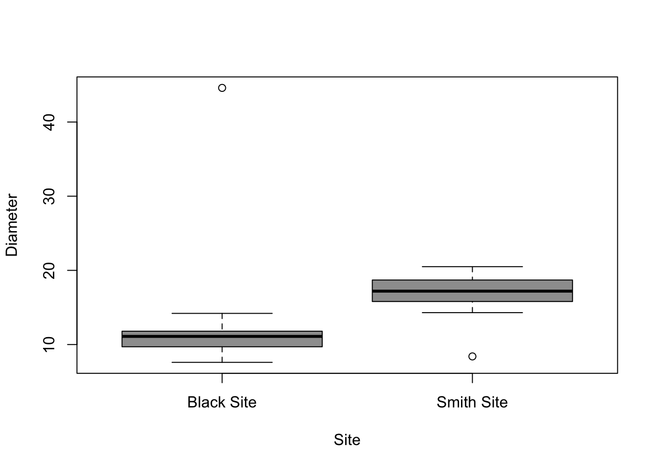
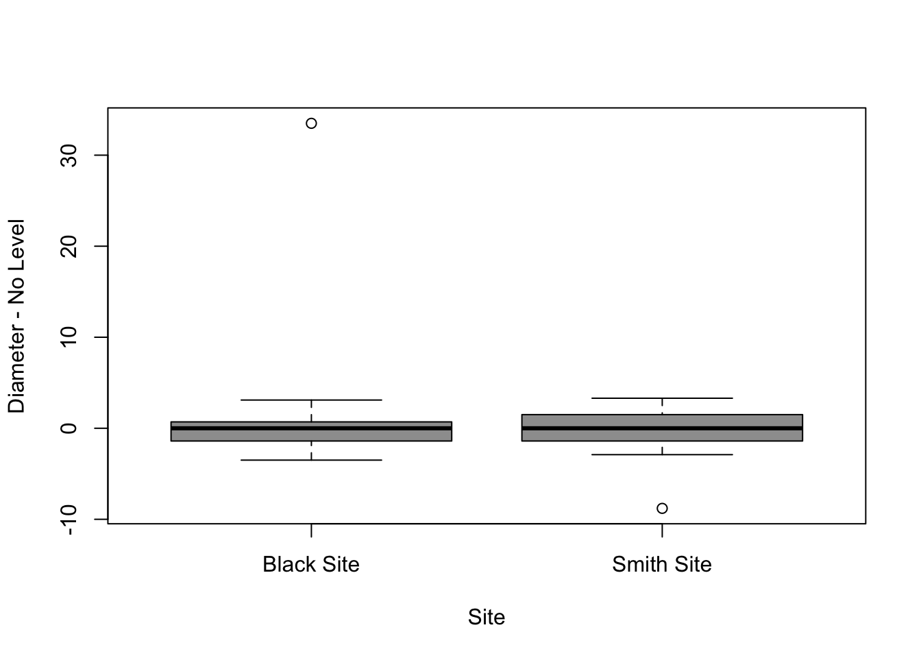
Drennan highlights the fact that there are multiple aspects of post-hole diameters that we might want to compare. The two sites clearly have different median post-hole diameters. But what if we want to compare the distributions of post-hole diameters at each site? To remove the level, we calculate the median post-hole diameter for each site, and then subtract that from each value (asking, in effect, “how far is each value from the median for that site?”).
#calculate the median diameter for each site
Smith_PostMed <- median(BSPosts[BSPosts$Site=="Smith Site",]$Diameter)
Black_PostMed <- median(BSPosts[BSPosts$Site=="Black Site",]$Diameter)
Smith_PostMed
## [1] 17.2## [1] 11.1#subtract the appropriate median from each value
BSPosts$nolevel <- ifelse(BSPosts$Site=="Black Site", BSPosts$Diameter - Black_PostMed,
BSPosts$Diameter - Smith_PostMed) Here we have used ifelse() to create a new column by subtracting the appropriate median - if ‘Site’ is “Black Site”, then subtract 11.1 from the diameter; otherwise (i.e. if it’s “Smith Site”) subtract 17.2. The ifelse() function - check ?ifelse describes a test (“does the value of Site = ‘Black’?”), then specifies what to do if the test produces a true answer (if “yes”, then subtract Black_PostMed from the value in the ‘Diameter’ column) or a false one (if “no”, then subtract Smith_PostMed from the value in the ‘Diameter’ column). Keeping in mind the median values (Black = 11.1; Smith = Smith_PostMed), examine your results (the newly-calculated ‘nolevel’ column) and make sure that they make sense.
##         Site Diameter nolevel
## 1 Black Site      9.7    -1.4
## 2 Black Site      9.2    -1.9
## 3 Black Site     12.9     1.8
## 4 Black Site     11.4     0.3
## 5 Black Site      9.1    -2.0
## 6 Black Site     44.6    33.5
Then, to produce Drennan’s Fig. 4.3
The next step is to remove the spread by reducing it to one (dividing by the midspread).
We’ll do this for each site separately, looking at a more efficient way of standardizing in the process - using scale() rather than doing the calculations ourselves. Using scale() we can standardize by either the median and the IQR, or by the mean and the standard deviation (the latter are referred to as Z-scores).
#subset by site
BlPosts <- BSPosts[BSPosts$Site == "Black Site",]
#add the variable "Scaled"
BlPosts$Scaled <- scale(BlPosts$Diameter, center = median(BlPosts$Diameter),
                        scale = IQR(BlPosts$Diameter))
#add z-scores
BlPosts$Z <- scale(BlPosts$Diameter)

#and the same for the Smith Site
SmPosts <- BSPosts[BSPosts$Site == "Smith Site",]
SmPosts$Scaled <- scale(SmPosts$Diameter, center = median(SmPosts$Diameter),
                        scale = IQR(SmPosts$Diameter))
SmPosts$Z <- scale(SmPosts$Diameter)

#put the data back together
BSPosts <- data.frame(rbind(BlPosts, SmPosts))
#and examine it
head(BSPosts)
## Site Diameter nolevel Scaled Z
## 1 Black Site 9.7 -1.4 -0.6666667 -0.39186538
## 2 Black Site 9.2 -1.9 -0.9047619 -0.44438343
## 3 Black Site 12.9 1.8 0.8571429 -0.05574992
## 4 Black Site 11.4 0.3 0.1428571 -0.21330404
## 5 Black Site 9.1 -2.0 -0.9523810 -0.45488703
## 6 Black Site 44.6 33.5 15.9523810 3.27389390We can now build the two parts of Drennan’s Fig. 4.4.
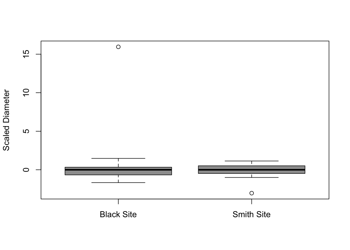
The empty quotes in xlab = "" specify that we don’t want to label the x-axis (it would be redundant, since we have labels for “Black Site” and “Smith Site”)
Then, to produce a reasonable approximation of the back-to-back stem-and-leaf plot that Drennan does:
## _____________________________
##   1 | 2: represents 1.2, leaf unit: 0.1
## BlPosts$Scaled
##                   SmPosts$Scaled
## _____________________________
##            | -4* |
##            | -3. |
##            | -3* |0      1
##            | -2. |
##            | -2* |
##    1      6| -1. |
##            | -1* |0      2
##    4    699| -0. |65     4
##    6     12| -0* |421    7
##   (4)  3210|  0* |0234  (4)
##    3      8|  0. |557    4
##    2      4|  1* |1      1
##            |  1. |
##            |  2* |
##            |  2. |
##            |  3* |
##            |  3. |
##            |  4* |
##            |  4. |
##            |  5* |
##            |  5. |
##            |  6* |
##            |  6. |
##            |  7* |
##            |  7. |
##            |  8* |
##            |  8. |
##            |  9* |
##            |  9. |
##            | 10* |
##            | 10. |
##            | 11* |
##            | 11. |
##            | 12* |
##            | 12. |
##            | 13* |
##            | 13. |
##            | 14* |
##            | 14. |
##            | 15* |
##    1      9| 15. |
##            | 16* |
## _____________________________
## n:       13       15
## _____________________________