1 Batches of Numbers (Ch. 1)
First re-create Table 1.8 Areas of 29 Sites in the Kiskiminetas River Valley. Although often you’ll read existing data into R, there are also various ways to build tables/datasets in R. Here we’ll use data.frame(), providing the name of the column/variable and the values with which to populate it. Note that adding more columns is as simple as adding another variable name and another set of values…but the number of values must match the first (tables can’t have ragged edges).
KRV <- data.frame(Area=c(12.8, 11.5, 14, 1.3, 10.3, 9.8, 2.3, 15.3, 11.2, 3.4, 12.8,
                         13.9, 9, 10.6, 9.9, 13.4, 8.7, 3.8, 11.7, 1.7, 12.3, 11,
                         2.9, 10.7, 7.4, 8.2, 2, 2.2, 4.5))
KRV
## Area
## 1 12.8
## 2 11.5
## 3 14.0
## 4 1.3
## 5 10.3
## 6 9.8
## 7 2.3
## 8 15.3
## 9 11.2
## 10 3.4
## 11 12.8
## 12 13.9
## 13 9.0
## 14 10.6
## 15 9.9
## 16 13.4
## 17 8.7
## 18 3.8
## 19 11.7
## 20 1.7
## 21 12.3
## 22 11.0
## 23 2.9
## 24 10.7
## 25 7.4
## 26 8.2
## 27 2.0
## 28 2.2
## 29 4.5Then produce a stem-and-leaf plot using these data…
##
##   The decimal point is at the |
##
##    1 | 37
##    2 | 0239
##    3 | 48
##    4 | 5
##    5 |
##    6 |
##    7 | 4
##    8 | 27
##    9 | 089
##   10 | 367
##   11 | 0257
##   12 | 388
##   13 | 49
##   14 | 0
##   15 | 3
…and a histogram.
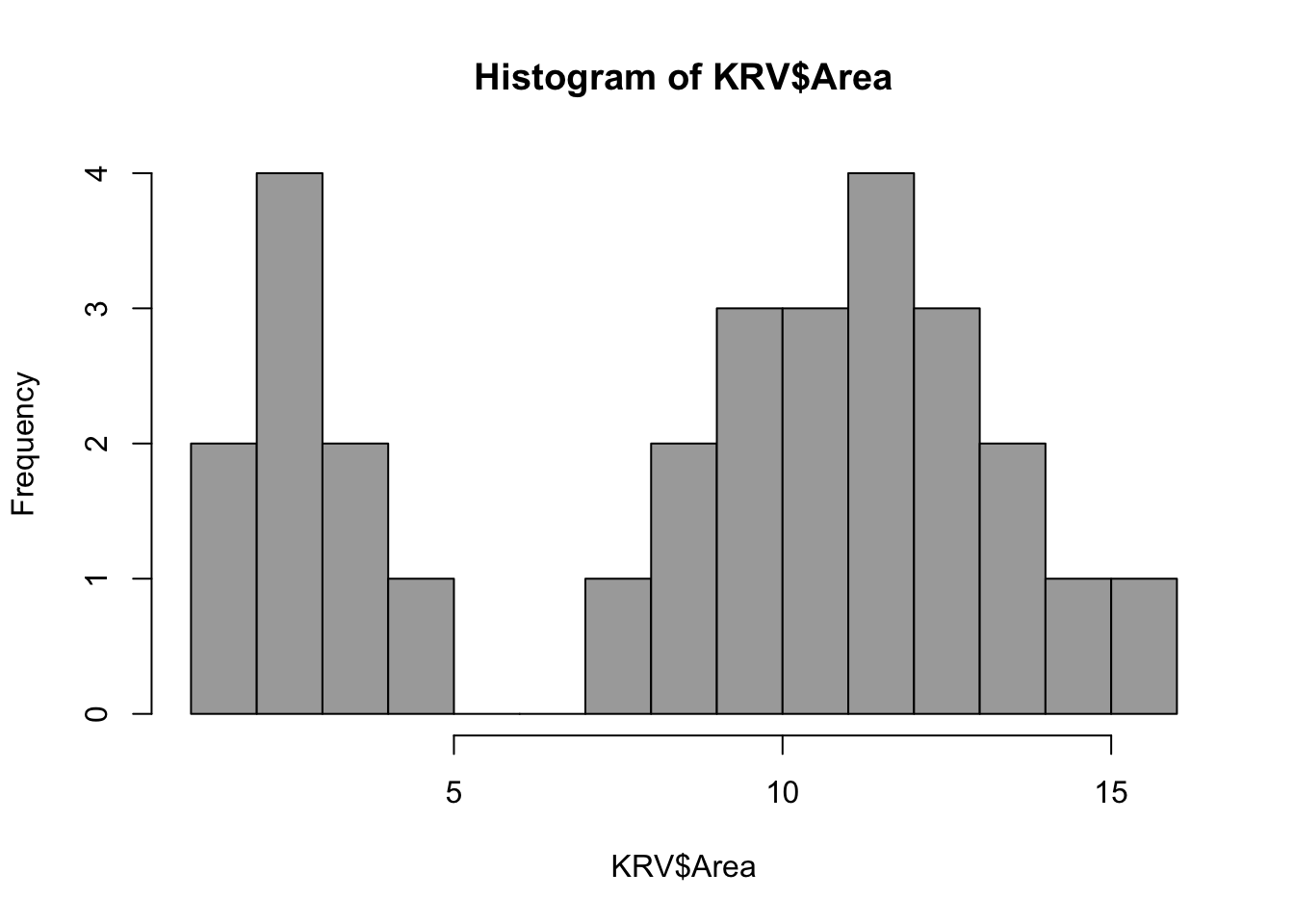
You’ve just recreated Drennan’s Fig. 1.2.
1.1 Import the Scraper data.
Download ‘scrapers.txt’. Often you’ll want to read an existing table (.xls, .csv, .txt, etc.) into R. Get used to figuring out where files live on your hard drive, and learn how to access the filepath (shift + rightclick on Windows; Option + Command + C on Mac). Note that the filepath can be either absolute (“where this lives on this machine”) or relative (“where this lives in this folder”). The former will never get lost (unless you move the file or rename folders), while the latter risks getting lost but is more portable.
You’ll use read.delim() for tab-delimited; read.table() or read.csv() are comparable for other data structures. (There are R packages that also enable reading data with more complex formats - Excel tables or Google sheets, most commonly.). Get used to examining the structure of any data file so that you can figure out how to use it (and about what specifically to curse the original author if necessary). There are various tricks for this - select + spacebar on a Mac, or TextEdit (included w/ the OS; TextWrangler and its spawn, BBEdit are free and better); on a PC try the free utility Notepad++.
Using - not to mention producing and maintaining - tabular data is a generally-overlooked but vital part of archaeological practice. One important advantage of working with data in R is that you can leave the original data file alone, instead making modifications to the objects you’re working with in R. This removes the risk - endemic to spreadsheet use - of corruption or loss of original data. Warning: making active use of tabular data will lead to you develop opinions about how one should manage such data (and there are in fact better and worse practices; for spreadsheets in particular see Broman and Woo (2018)). For notes on wrangling data in R, see here.
##               Site Material Length
## 1  Pine Ridge Cave    Chert   25.8
## 2  Pine Ridge Cave    Chert    6.3
## 3  Pine Ridge Cave    Flint   44.6
## 4  Pine Ridge Cave    Chert   21.3
## 5  Pine Ridge Cave    Flint   25.7
## 6  Pine Ridge Cave    Chert   20.6
## 7  Pine Ridge Cave    Chert   22.2
## 8  Pine Ridge Cave    Chert   10.5
## 9  Pine Ridge Cave    Chert   18.9
## 10 Pine Ridge Cave    Chert   25.9
## 11 Pine Ridge Cave    Chert   23.8
## 12 Pine Ridge Cave    Chert   22.0
## 13 Pine Ridge Cave    Chert   10.6
## 14 Pine Ridge Cave    Flint   33.2
## 15 Pine Ridge Cave    Chert   16.8
## 16 Pine Ridge Cave    Chert   21.8
## 17 Pine Ridge Cave    Flint   48.3
## 18    Willow Flats    Chert   15.8
## 19    Willow Flats    Flint   39.4
## 20    Willow Flats    Flint   43.5
## 21    Willow Flats    Flint   39.8
## 22    Willow Flats    Chert   16.3
## 23    Willow Flats    Flint   40.5
## 24    Willow Flats    Flint   91.7
## 25    Willow Flats    Chert   21.7
## 26    Willow Flats    Chert   17.9
## 27    Willow Flats    Flint   29.3
## 28    Willow Flats    Flint   39.1
## 29    Willow Flats    Flint   42.5
## 30    Willow Flats    Flint   49.6
## 31    Willow Flats    Chert   13.7
## 32    Willow Flats    Chert   19.1
## 33    Willow Flats    Flint   40.6
## 34    Willow Flats    Flint   49.1
## 35    Willow Flats    Flint   41.7
## 36    Willow Flats    Chert   15.2
## 37    Willow Flats    Chert   21.2
## 38    Willow Flats    Flint   30.2
## 39    Willow Flats    Flint   40.0
## 40    Willow Flats    Chert   20.2
## 41    Willow Flats    Flint   31.9
## 42    Willow Flats    Flint   42.3
## 43    Willow Flats    Flint   47.2
## 44    Willow Flats    Flint   50.5
## 45    Willow Flats    Chert   10.6
## 46    Willow Flats    Chert   23.1
## 47    Willow Flats    Flint   44.1
## 48 Willow Flats Flint 45.8##
## The decimal point is 1 digit(s) to the right of the |
##
## 0 | 6
## 1 | 11145667899
## 2 | 01112222346669
## 3 | 02399
## 4 | 00112234456789
## 5 | 01
## 6 |
## 7 |
## 8 |
## 9 | 2An alternative (in R there are often several) stem-and-leaf plot is available from the package ‘aplpack’. Install this package using either R-Studio’s convenient interface or the command line.
#uncomment the below to run this line
# install.packages("aplpack", repos="https://cran.rstudio.com/")
Alternatively, in R Studio, use the ‘Install’ command in the ‘Packages’ tab of the ‘Files / Plots / Packages / Help’ pane. Then you can load the package (and R will automatically load any other packages upon which this one depends):
Then you can use the functions that are available in that package, e.g.:
## 1 | 2: represents 12
##  leaf unit: 1
##             n: 48
##    1    0. | 6
##    5    1* | 0003
##   12    1. | 5566789
##   22    2* | 0011112233
##   (4)   2. | 5559
##   22    3* | 013
##   19    3. | 999
##   16    4* | 000122344
##    7    4. | 57899
##    2    5* | 0
## HI: 91.7
You can also run an individual function from a package without loading that package by specifying the package when you call the function:
## 1 | 2: represents 12
##  leaf unit: 1
##             n: 48
##    1    0. | 6
##    5    1* | 0003
##   12    1. | 5566789
##   22    2* | 0011112233
##   (4)   2. | 5559
##   22    3* | 013
##   19    3. | 999
##   16    4* | 000122344
##    7    4. | 57899
##    2    5* | 0
## HI: 91.7
You may want to know just how stem.leaf() is different than stem(). Remember that ? is always an option, and should be used early and often.
With the data in hand and having looked at it in aggregate, it may be useful to expore it further, for instance by spliting the batch by site and/or by material and examining it again.
#make two subsets, by site
PRCscrapers <- subset(scrapers, Site == "Pine Ridge Cave")
# here these are subsetted and assigned to a new object
PRCscrapers #which you can examine
## Site Material Length
## 1 Pine Ridge Cave Chert 25.8
## 2 Pine Ridge Cave Chert 6.3
## 3 Pine Ridge Cave Flint 44.6
## 4 Pine Ridge Cave Chert 21.3
## 5 Pine Ridge Cave Flint 25.7
## 6 Pine Ridge Cave Chert 20.6
## 7 Pine Ridge Cave Chert 22.2
## 8 Pine Ridge Cave Chert 10.5
## 9 Pine Ridge Cave Chert 18.9
## 10 Pine Ridge Cave Chert 25.9
## 11 Pine Ridge Cave Chert 23.8
## 12 Pine Ridge Cave Chert 22.0
## 13 Pine Ridge Cave Chert 10.6
## 14 Pine Ridge Cave Flint 33.2
## 15 Pine Ridge Cave Chert 16.8
## 16 Pine Ridge Cave Chert 21.8
## 17 Pine Ridge Cave Flint 48.3WFscrapers <- subset(scrapers, Site == "Willow Flats")
#back-to-back stem and leaf plot to easily compare the two sites visually
stem.leaf.backback(PRCscrapers$Length,WFscrapers$Length, trim.outliers = F)## ____________________________________________
## 1 | 2: represents 12, leaf unit: 1
## PRCscrapers$Length WFscrapers$Length
## ____________________________________________
## 1 6| 0 |
## 5 8600| 1 |0355679 7
## (9) 555322110| 2 |01139 12
## 3 3| 3 |01999 (5)
## 2 84| 4 |000122345799 14
## | 5 |0 2
## | 6 |
## | 7 |
## | 8 |
## | 9 |1 1
## | 10 |
## ____________________________________________
## n: 17 31
## ____________________________________________Reordering data can also be a useful exploratory tool.
##               Site Material Length
## 2  Pine Ridge Cave    Chert    6.3
## 8  Pine Ridge Cave    Chert   10.5
## 13 Pine Ridge Cave    Chert   10.6
## 15 Pine Ridge Cave    Chert   16.8
## 9  Pine Ridge Cave    Chert   18.9
## 6  Pine Ridge Cave    Chert   20.6
## 4  Pine Ridge Cave    Chert   21.3
## 16 Pine Ridge Cave    Chert   21.8
## 12 Pine Ridge Cave    Chert   22.0
## 7  Pine Ridge Cave    Chert   22.2
## 11 Pine Ridge Cave    Chert   23.8
## 5  Pine Ridge Cave    Flint   25.7
## 1  Pine Ridge Cave    Chert   25.8
## 10 Pine Ridge Cave    Chert   25.9
## 14 Pine Ridge Cave    Flint   33.2
## 3  Pine Ridge Cave    Flint   44.6
## 17 Pine Ridge Cave    Flint   48.3
## 45    Willow Flats    Chert   10.6
## 31    Willow Flats    Chert   13.7
## 36    Willow Flats    Chert   15.2
## 18    Willow Flats    Chert   15.8
## 22    Willow Flats    Chert   16.3
## 26    Willow Flats    Chert   17.9
## 32    Willow Flats    Chert   19.1
## 40    Willow Flats    Chert   20.2
## 37    Willow Flats    Chert   21.2
## 25    Willow Flats    Chert   21.7
## 46    Willow Flats    Chert   23.1
## 27    Willow Flats    Flint   29.3
## 38    Willow Flats    Flint   30.2
## 41    Willow Flats    Flint   31.9
## 28    Willow Flats    Flint   39.1
## 19    Willow Flats    Flint   39.4
## 21    Willow Flats    Flint   39.8
## 39    Willow Flats    Flint   40.0
## 23    Willow Flats    Flint   40.5
## 33    Willow Flats    Flint   40.6
## 35    Willow Flats    Flint   41.7
## 42    Willow Flats    Flint   42.3
## 29    Willow Flats    Flint   42.5
## 20    Willow Flats    Flint   43.5
## 47    Willow Flats    Flint   44.1
## 48    Willow Flats    Flint   45.8
## 43    Willow Flats    Flint   47.2
## 34    Willow Flats    Flint   49.1
## 30    Willow Flats    Flint   49.6
## 44    Willow Flats    Flint   50.5
## 24 Willow Flats Flint 91.7## Site Material Length
## 2 Pine Ridge Cave Chert 6.3
## 8 Pine Ridge Cave Chert 10.5
## 13 Pine Ridge Cave Chert 10.6
## 45 Willow Flats Chert 10.6
## 31 Willow Flats Chert 13.7
## 36 Willow Flats Chert 15.2
## 18 Willow Flats Chert 15.8
## 22 Willow Flats Chert 16.3
## 15 Pine Ridge Cave Chert 16.8
## 26 Willow Flats Chert 17.9
## 9 Pine Ridge Cave Chert 18.9
## 32 Willow Flats Chert 19.1
## 40 Willow Flats Chert 20.2
## 6 Pine Ridge Cave Chert 20.6
## 37 Willow Flats Chert 21.2
## 4 Pine Ridge Cave Chert 21.3
## 25 Willow Flats Chert 21.7
## 16 Pine Ridge Cave Chert 21.8
## 12 Pine Ridge Cave Chert 22.0
## 7 Pine Ridge Cave Chert 22.2
## 46 Willow Flats Chert 23.1
## 11 Pine Ridge Cave Chert 23.8
## 1 Pine Ridge Cave Chert 25.8
## 10 Pine Ridge Cave Chert 25.9
## 5 Pine Ridge Cave Flint 25.7
## 27 Willow Flats Flint 29.3
## 38 Willow Flats Flint 30.2
## 41 Willow Flats Flint 31.9
## 14 Pine Ridge Cave Flint 33.2
## 28 Willow Flats Flint 39.1
## 19 Willow Flats Flint 39.4
## 21 Willow Flats Flint 39.8
## 39 Willow Flats Flint 40.0
## 23 Willow Flats Flint 40.5
## 33 Willow Flats Flint 40.6
## 35 Willow Flats Flint 41.7
## 42 Willow Flats Flint 42.3
## 29 Willow Flats Flint 42.5
## 20 Willow Flats Flint 43.5
## 47 Willow Flats Flint 44.1
## 3 Pine Ridge Cave Flint 44.6
## 48 Willow Flats Flint 45.8
## 43 Willow Flats Flint 47.2
## 17 Pine Ridge Cave Flint 48.3
## 34 Willow Flats Flint 49.1
## 30 Willow Flats Flint 49.6
## 44 Willow Flats Flint 50.5
## 24 Willow Flats Flint 91.7Note that since we are not writing these to an object, the result is only temporary (we have not altered ‘scrapers’ nor assigned the re-ordered data to a new object).
Subsetting by material can also be useful.
chertscrapers <- subset(scrapers, Material == "Chert")
# here the results *are* assigned to a new object, which you can then examine
chertscrapers
## Site Material Length
## 1 Pine Ridge Cave Chert 25.8
## 2 Pine Ridge Cave Chert 6.3
## 4 Pine Ridge Cave Chert 21.3
## 6 Pine Ridge Cave Chert 20.6
## 7 Pine Ridge Cave Chert 22.2
## 8 Pine Ridge Cave Chert 10.5
## 9 Pine Ridge Cave Chert 18.9
## 10 Pine Ridge Cave Chert 25.9
## 11 Pine Ridge Cave Chert 23.8
## 12 Pine Ridge Cave Chert 22.0
## 13 Pine Ridge Cave Chert 10.6
## 15 Pine Ridge Cave Chert 16.8
## 16 Pine Ridge Cave Chert 21.8
## 18 Willow Flats Chert 15.8
## 22 Willow Flats Chert 16.3
## 25 Willow Flats Chert 21.7
## 26 Willow Flats Chert 17.9
## 31 Willow Flats Chert 13.7
## 32 Willow Flats Chert 19.1
## 36 Willow Flats Chert 15.2
## 37 Willow Flats Chert 21.2
## 40 Willow Flats Chert 20.2
## 45 Willow Flats Chert 10.6
## 46 Willow Flats Chert 23.1flintscrapers <- subset(scrapers, Material == "Flint")
#back-to-back stem and leaf plot
stem.leaf.backback(chertscrapers$Length, flintscrapers$Length, trim.outliers = F)## __________________________________________________
## 1 | 2: represents 12, leaf unit: 1
## chertscrapers$Length flintscrapers$Length
## __________________________________________________
## 1 6| 0 |
## (11) 98766553000| 1 |
## (12) 553322111100| 2 |59 2
## | 3 |013999 8
## | 4 |00012234457899 (14)
## | 5 |0 2
## | 6 |
## | 7 |
## | 8 |
## | 9 |1 1
## | 10 |
## __________________________________________________
## n: 24 24
## __________________________________________________#note that this could also be accomplished without creating new objects
stem.leaf.backback(subset(scrapers, Material == "Chert")$Length,
subset(scrapers, Material == "Flint")$Length, trim.outliers = F)## __________________________________________________
## 1 | 2: represents 12, leaf unit: 1
## subset(scrapers, Material == "Chert")$Length
## subset(scrapers, Material == "Flint")$Length
## __________________________________________________
## 1 6| 0 |
## (11) 98766553000| 1 |
## (12) 553322111100| 2 |59 2
## | 3 |013999 8
## | 4 |00012234457899 (14)
## | 5 |0 2
## | 6 |
## | 7 |
## | 8 |
## | 9 |1 1
## | 10 |
## __________________________________________________
## n: 24 24
## __________________________________________________